The functionality of a part in an assembly is usually well defined by the 4 form tolerances (straigthness, flatness, circularity and cylindricity) and among the orientation tolerances by the 3 most frequent ones: the position, the perpendicularity and the parallelism tolerance.
Yet we have 14 different types of tolerances in total, which can be anytime used to accuratelly define how a part/ assembly of parts will work. Not all these are also easy to measure, and in some cases things can become really complex. Therefore instead of working with difficult to measure characteristics, it is better to use as many as necessary simple ones.
In my previous articles I’ve already talked about the most used tolerances. In this article I want to focus on the Concentricity tolerance which is probably the most difficult to measure, but in some special cases is it good to specify it.
Note: Concentricity was removed from the 2018 ASME Y14.5 standard. It is still commonly in use for those on previous versions of the standard.
Description
The terms coaxiality and concentricity are sometimes used with the same meaning. Strictly speaking, bodies of revolution with the same axis are coaxial, while two circles that lie in one plane and have the same center point are concentric. But coaxiality is the more comprehensive term, which is why we usually use it. The difference is not important.
However, this is important for most technical rotating parts, e.g. gear shafts or coupling housings, to limit the axis deviation. The dimensional tolerance does not include any coaxiality tolerance. There is also not simply “the” axis of a shaft, rather it must be specified exactly how the reference axis is to be formed.
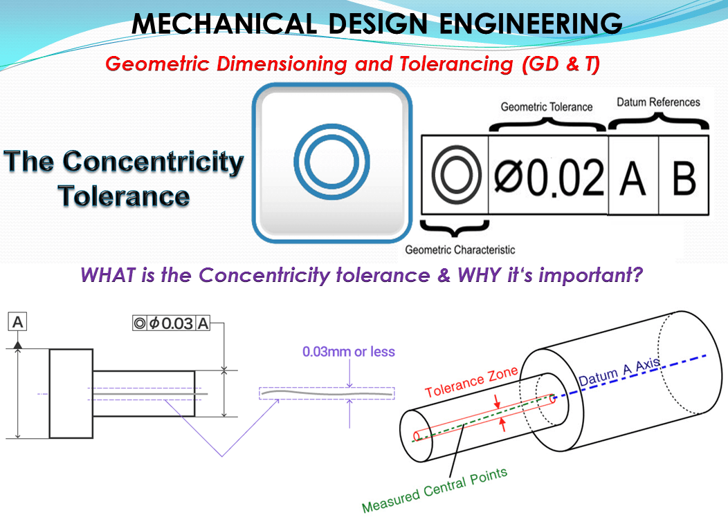
Concentricity, (called coaxiality in the ISO Standard), is: a tolerance that controls the central derived median points of the referenced feature, to a datum axis.
Concentricity is in fact a special case of Positon tolerance.
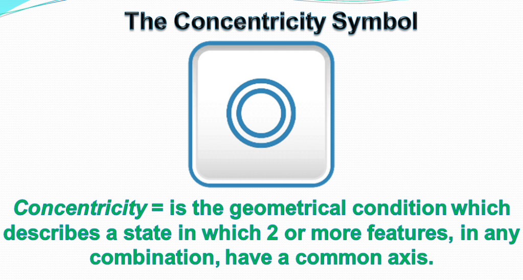
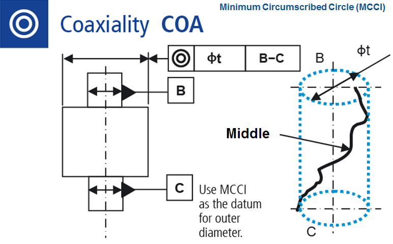
Symbol: –The symbol of concentricity tolerance are 2 concentric circles (as shown in figure 1.) This symbol is specified in the left compartment of the feature control frame and it is used to describe measurements from derived median points as opposed to a surface or feature’s axis.
The Tolerance call out: Concentricity = Toleranced and datum elements are always axis or center points of rotational elements, which means that tolerance arrow or reference triangle are always on the coresponding diameter dimension arrow.
The nominal axis of a tolerated element is derived from individual cross-sections, for intance it can be crooked. A limited case is the concenticity of spheres.

How does it work?
As I’ve already mentioned Coaxiality is the relationship between multiple cylindrical or revolute features sharing a common axis. Coaxiality can be specified in several different ways, using a runout, concentricity, or positional tolerance.
For instance a runout tolerance controls surface deviations directly, without regard for the feature’s axis. Yet a concentricity tolerance, controls the midpoints of diametrically opposed points.
The standards don’t have a name for the relationship between multiple width-type features sharing a common center plane. I will extend the term coplanarity to apply in this context. Coplanarity can be specified using either a symmetry or positional tolerance. A symmetry tolerance, controls the midpoints of opposed surface points. Where one of the coaxial or coplanar features is identified as a datum feature, the coaxiality or coplanarity of the other(s) can be controlled directly with a positional tolerance applied at RFS (Regardless of Feature Size), MMC, or LMC. Likewise, the datum reference can apply at RFS, MMC, or LMC. For each controlled feature, the tolerance establishes either a virtual condition boundary or a central tolerance zone located at true position. In this case, no basic dimensions are expressed, because true position is coincident with the referenced datum axis or datum center plane.
All the above principles can be extended to a pattern of coaxial feature groups. For a pattern of counterbored holes, the pattern of holes is located as usual. A single “datum feature” symbol is attached. Coaxiality for the counterbores is specified with a separate feature control frame. In addition, a note such as for instance 4X INDIVIDUALLY is placed under the “datum feature” symbol and under the feature control frame for the counterbores, indicating the number of places each applies on an individual basis.
Where the coaxiality or coplanarity of two features is controlled with a positional tolerance of zero at MMC and the datum is also referenced at MMC, it makes no difference which of these features is the datum. For each feature, its TGC (True Geometric Counterpart), its virtual condition, and its MMC size limit are identical. The same is true in an all-LMC context.
Tolerance zone
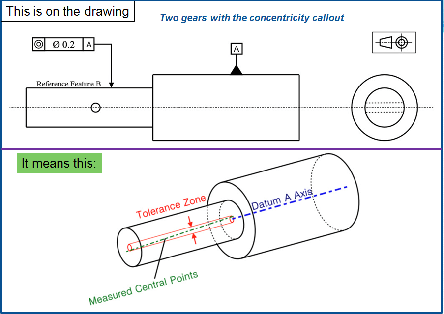
Concentricity is a 3-Dimensional cylindrical tolerance zone that is defined by a datum axis where all the derived median points of a referenced cylindrical feature must fall within. All median points along the entire feature must be in this tolerance zone.
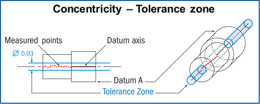
The concentricity tolerance zone is always circular (with diameter symbol Ø in the tolerance frame) and is coaxial with the reference axis. The limit deviation as the largest permissible axis offset, is half of the concentricity tolerance tCO/2.
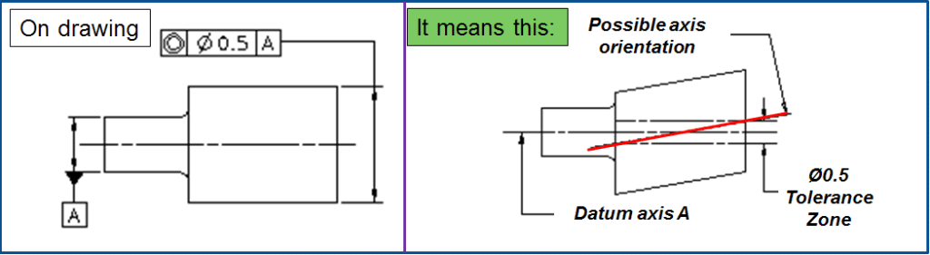
Hence if the largest permissible axis offset is specified the concenticity tolerance can be twice as large. From the tubular shaped tolerance zone results that for included deviations, the straightness deviations of the tolerated axis and its paralellism deviation from the reference axis can not be bigger than concentricity tolerance tCO.
On the other hand roundness and cylindricity tolerance affect the outer surface of the tolerated element which have nothing to do with concentricity.
This type of tolerancing is also neither functional – because the 2 bearing seats are treated very unequally and this allows too large deviation from the tolerated feature – nor test-compliant due to its measurement uncertainity. However if it mostly fulfills its purpose in practice, then the reason is that an experienced production worker will manufacture the 2 bearing seats in one clamping in view of such tolerance, so that sufficient allignment is usually guaranteed with an intact cylindrical grinding machine. But this cannot be a justificaton for such a tolerance type.
For this reason, a good recommendation applicable in this case as a guideline is the following rule:
Reference extentions: If the reference datum and the tolerated element are spatially apart, so that the reference must be extended to the toleranced element, then the measurement uncertainity increases approximativelly in relation to the average distance between reference datum and the tolerated element on the length l of the reference element. You should then not exceed a ratio of a/l ≈ 2 (as guideline) (as shown in the example 5 (b) in FIG. 10 below)
This rule also applies to median planes or real surface references: Not only when the distance a is too big but it should be generally applied as common toleance zone (CZ).
When is the Concentricity/Coaxiality tolerance used?
Due to its complex nature, Concentricity is usually reserved for parts that require a high degree of precision to function properly. Transmission gears, which need to always be coaxial to avoid oscillations and wear, may require concentricity to ensure all the axes line up correctly. Equal mass or inertial concerns are one of the leading causes for the concentricity callout, however are often better designed with runout. In fact, in most cases, the use of runout or position should replace the need for concentricity and be much easier to measure.
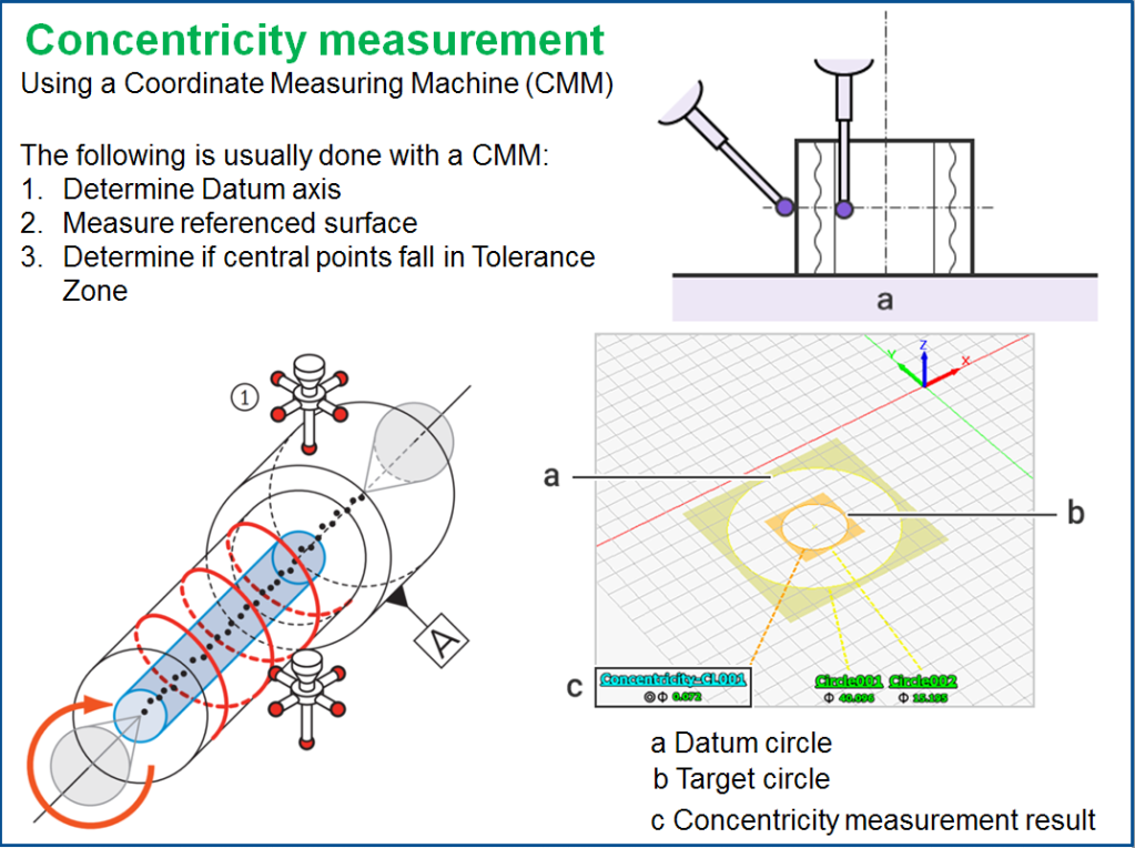
Concentricity example of use: As shown in FIG 6, An intermediate shaft in a transmission is composed of two different cylindrical sections which are coaxial. Datum A (right) is the drive side and relatively fixed with bearings to the housing, The referenced surface B is desired to be concentric with Datum A to avoid oscillations at high speed.
Concentricity would require side B to be measured in all dimensions several times to obtain a full dimensional scan of the surface of the reference feature. This scan must then be analyzed to determine the derived median points at each location along the cylinder fall within the tolerance zone. The tolerance zone would be established by the datum axis derived from datum feature A. All central points would all need to fall into the cylindrical tolerance zone to be in tolerance. This would all be done with a CMM and measurement software and required special measurement programs to compare the axes.
In this example, the measured derived median points (green) all fall within the cylindrical tolerance zone surrounding datum axis A, ensuring a smooth, near-perfect rotational system. Note that the derived median points do not need to form a straight line and may be scattered due to imperfections in the surface. However, as long as they all fall within the tolerance zone the part is in spec.
Let’s see now some of the most frequent examples of use for concentricity tolerace:
Example 1. Concentricity tolerancing of a revolute
As illustrated in Fig. 7, a revolute feature is one of the most common applications of symmetry tolerancing.
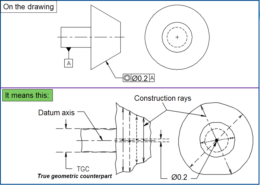
In Fig. 7 this is specified by a feature control frame containing the “concentricity” symbol. In this special symmetry case, the datum is an axis. There are two rays 180° apart (colinear) perpendicular to the datum axis. The rays intersect the feature surface at two diametrically opposed points. The midpoint between those two surface points shall lie within a cylindrical tolerance zone coaxial to the datum and having a diameter equal to the concentricity tolerance value. At each cross-sectional slice, the revolving rays generate a locus of distinct midpoints. As the rays sweep the length of the controlled feature, these 2-D loci of midpoints stack together, forming a 3-D “wormlike” locus of midpoints. The entire locus shall be contained within the concentricity tolerance cylinder. Don’t confuse this 3-D locus with the 1D derived median line defined for median line (applied for Straightness) or median plane (applied for Flatness)
Example 2. Concentricity Tolerance for Multifold Symmetry about a Datum Axis
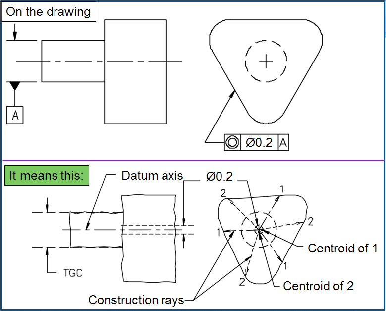
The explanation of concentricity in Y14.5 standard is somewhat abstruse because it’s also meant to support multifold symmetry about an axis. Any prime number of rays can be projected perpendicular from the datum axis, provided they are coplanar with equal angular spacing. For the 3-lobe cam in Fig. 8, there are three rays, 120° apart. A 25-blade impeller would require five rays spaced 72° apart, etc. From the multiple intersection points, a centroid is then constructed and checked for containment within the tolerance zone. The standards don’t specify how to derive the centroid, but I recommend the Minimum Radial Separation (MRS) method described in ANSI B89.3.1-1972. Obviously, verification is well beyond the capability of an inspector using multiple indicators and a calculator. Notice that as the rays are revolved about the datum axis, they intersect the surface(s) at vastly different distances from center. Nevertheless, if the part is truly symmetrical, the centroid still remains within the tolerance cylinder.
Example 3. Concentricity Tolerance about a Datum Point
The “concentricity” symbol can also be used to specify twofold or multifold symmetry about a datum point. This could apply to a sphere, tetrahedron, dodecahedron, etc. In all cases, the basic geometry defines the symmetry rays, and centroids are constructed and evaluated. The tolerance value is preceded by the symbol S, specifying a spherical tolerance zone.
Example 4. Concentricity on single axis

a) Shaft heel with long reference axis: = The datum A is the axis of the left shaft heel. The tolerance zone of Ø0,1 mm limits the offset, the parallelism and the straightness of the axis of the right heel.
b) Bearing seat with “short” reference axis: = the axis of the bearing seat Ø30 H7 is defined by flange A and central axis B.
c) Washer concentricity: = Likewise in this case the primary datum A defines the measurement direction. The reference and tolerated element can also be swapped, depending on functionality.
Example 5. Concentricity on 2 axes
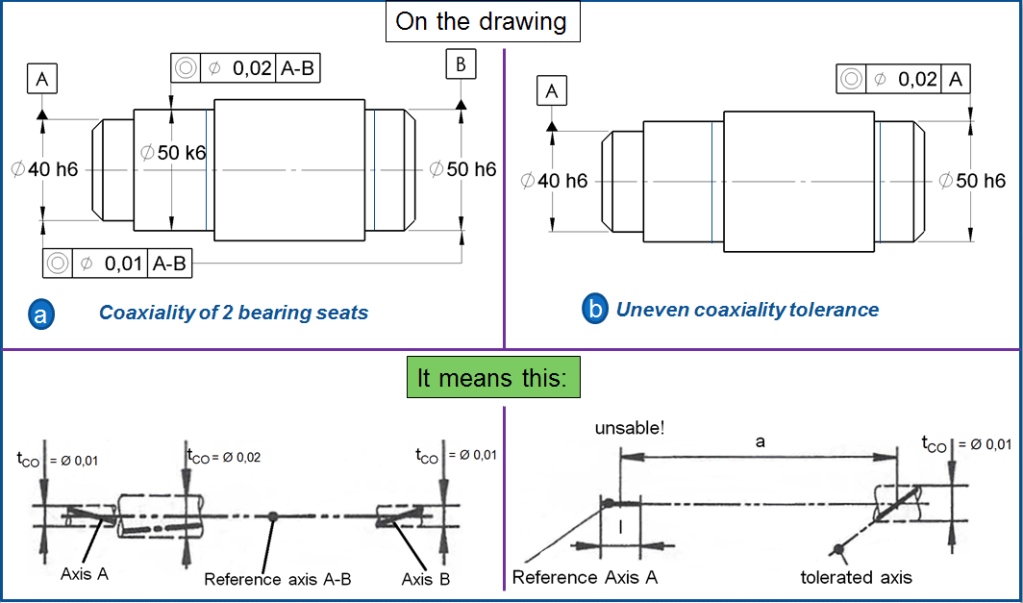
a) Coaxiality of 2 bearing seats = In this case we deal with a so called “floating” coaxiality because the 2 bearing seats must be relativelly aligned with each other (comparable with the example of floating holes as mentioned in my previous post for Position tolerance). Yet, a coaxiality without a reference input it won’t be acceptable for the measuring device, that’s why the common axis of the 2 bearing seats is taken as A-B reference. During the measurement the equipment first scans the 2 outer surfaces of the bearing seats, then from this derives the individual axis A and B, forms a common reference axis from the 2, places the 2 tubular tolerance zones of Ø0,01 around the common reference A-B and checks if the individual axis lie within these tubular tolerance zones. This procedure is especially useful if the measuring device has to form the axis A-B anyway, for the coaxiality tolerance of Ø0.02 mm.
b) Uneven coaxiality tolerance = In practice we often encounter this type of tolerancing instead of that mentioned at example a – FIG 10. As structure it somehow comforms with the Example N°4 in Fig 9(a) but in this case such structure is useless. The measuring gauge at first finds the reference axis A of the left seat and then extends it to about 8 folds to the right side where there is the tolerance zone of Ø0,02 mm.This also increase the measurement uncertainity by a factor of 8. Even a small deviation in the calculation of the axis or for the position of the reference datum A can result a tolerated element being outside of tolerance zone. But however this is linked to reference element not to the tolerated element. While the reference element must be preciselly alligned in the direction of toleranced element, so that the tolerance is mantained, the tolerance element can exhaust its tolerance zone and can be for instance crooked with 0.02mm. If you have coaxiality requirements for the bearing seat on the left then this doesn’t apply for the bearing seat on the right side. Due to the measurement uncertainity a constraint of coaxiality tolerance of tCO = Ø0,01 mm is also out to dicussion.
Gauging / Measurement
Concentricity is considered one of the most difficult GD&T symbols to measure, due to its difficulty in establishing the midpoints of the feature. First, you must establish a datum axis which to measure. Once the datum axis is established you must take measure many of a series of cross-sections (however many is realistic) to establish “diametrically opposed” surface points (surface points directly opposite from each other across the diameter). The median points of these diametrically opposed surface points must then be mapped out for the entire feature. Finally, these points are compared to the tolerance zone established by the datum axis. This can only be done on a CMM or other computer measurement device and is quite time-consuming.
However if the measurement is done using a dial gauge then you must hold the target in place and put the dial gauge on the vertex of the circumference for the axis for which tolerance is indicated. Rotate the target and measure the maximum and minimum run-out values using the dial gauge. Measure around the specified circumference. The greatest maximum-minimum difference is used as the concentricity.

DISADVANTAGES = Factors such as the angle and strength used to put the dial gauge on the target affect the measured value, which implies that measurements may differ depending on the operator. The friction between the tip of the dial gauge and the surface of the target may also leave scratches on the surface of the target.
In case of using a CMM unlike with coaxiality, you measure the circle of the plane.
For this measuring method you must put the stylus on the measurement point on the datum circle, and then put the stylus on the measurement point on the target circle to measure the concentricity. The stylus only comes into light contact with the surface and does not scratch the target.
For an accurate Coaxiality checking: A direct mechanical measurement is not possible. Form-testing devices determine the coaxiality deviation via a circular run-out measurement. A general problem with this, is which method is used in order to calculate the nominal axis. (for more about axis and middle plane as reference datums, I’ll share in another article).
To date there is no uniform or standardized specification for this. It’s to be expected that as part of the standardization project “Geometric Product Specification” the coresponding measuring methods to be defined and standardized. If no measurement device is avalable then instead of concentricity it’s better to tolerate the circular run-out since this can be directly measured. (see the article about circular runout). However besides that another problem arises, namely:
The Included tolerance at circular run-out = In the run-out tolerance tCR the circularity (roundness) tolerance tR with the same tolerance value is included, yet the concentricity tolerance tCO is only with an exceeding factor Ef. Currently this appears to be around 1.2 as usable value, but not Ef=1 as is often is assumed.
For a Circular run-out and concentricity checking: if instead of referenced concentricity tolerance tCO, the circular run-out is measured, then permissible run-out deviation dRO the following formula applies:
dRO ≤≈tCO/Ef
with Ef≈1,2 (for more clarity on this I’ll explain in the article about Circular Run-Out tolerance)
Relation to other GD & T Symbols
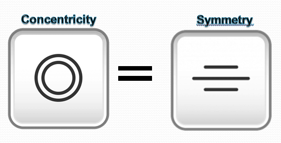
Concentricity is considered the “circular” form of GD & T symmetry.
While symmetry measures the true midpoint plane of a feature to a datum plane or axis, concentricity measures the derived midpoint axis to a datum axis. Both are notoriously difficult to measure.
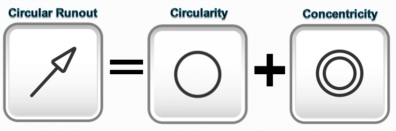
Runout is a combination control that can indirectly control concentricity and circularity simultaneously.
e.g.= If a part is perfectly round (perfect circularity), the runout measurement will equal the concentricity, if the part is perfectly centered (perfect concentricity) the runout will equal the circularity.
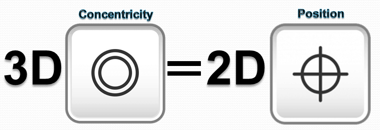
Concentricity is also a 3D form of 2-Dimensional True Position when applied to a circular feature.
While true position is usually controlled to a fixed point in space that forms from coordinate measurements from a datum (perfectly straight) of the feature, concentricity is controlled to the axis derived from an all the median points (imperfect and scattered) of a datum surface or feature.
Final Notes
Avoid Concentricity! : You will always hear from most machinists, measurement techs and designers to avoid concentricity like the plague. Unless it is absolutely necessary to control the distribution of mass around a part’s median points you should look to other more applicable GD &T Symbols. A good replacement for concentricity is circular runout since it relates the surface of a feature to a datum axis, while concentricity relates the derived axis to said datum. You can physically touch and measure the surface of the part to obtain a runout measurement. Controlling runout will also control the concentricity, albeit at a lesser extent than when concentricity is applied on its own. (Runout tolerance > Concentricity because Runout = Concentricity + Circularity).
Use in ammunition measurement: Often you will see concentricity gauges that are applied to homemade bullet casings. These gauges, however, do not measure concentricity by actually measure runout. However, since runout is just a combination of circularity and concentricity, you can technically say that you are measuring the concentricity of the bullet.
FAQ: Where a piston’s ring grooves interrupt the outside diameter (OD), do I need to control coaxiality among the three separate segments of the OD?
A: If it weren’t for those pesky grooves, Rule #1 would impose a boundary of perfect form at MMC for the entire length of the piston’s OD. Instead of using 3X to specify multiple same-size ODs, place the note THREE SURFACES AS A SINGLE FEATURE adjacent to the diameter dimension. That forces Rule #1 to ignore the interruptions. A similar note can simplify orientation and/or location control of a pattern of coaxial or coplanar same-size features.
According to ASME Y14.5M-1994, the Rule #1 decrees that: “Where only a tolerance of size is specified, the limits of size of an individual feature prescribe the extent to which variations in its form—as well as in its size—are allowed”
FAQ: Since a runout tolerance includes concentricity control and is easier to check, wouldn’t it save money to replace every concentricity tolerance with an equal runout tolerance? We wouldn’t need concentricity at all.
A: Though that is the policy at many companies, there’s another way to look at it. Let’s consider a design where significant out-of-roundness can be tolerated as long as it’s symmetrical. A concentricity tolerance is carefully chosen. We can still use runout’s FIM (Full Indicator Movement) method to inspect a batch of parts. Of those conforming to the concentricity tolerance, all or most parts will pass the FIM test and be accepted quickly and cheaply. Those few parts that fail the FIM inspection may be reinspected using the formal concentricity method. The concentricity check is more elaborate and expensive than the simple FIM method, but also more forgiving, and would likely accept many of the suspect parts. Alternatively, management may decide it’s cheaper to reject the suspect parts without further inspection and to replace them. The waste is calculated and certainly no worse than if the well-conceived concentricity tolerance had been arbitrarily converted to a runout tolerance. The difference is this: If the suspect parts are truly usable, the more forgiving concentricity tolerance offers a chance to save them.

Nice illustration
LikeLike