
Runout is one of the oldest and simplest concepts used in GD & T. Maybe as a child you stood your bicycle upside down on the ground and spun a wheel. If you fixed your stare on the shiny rim where it passed a certain part of the frame, you could see the rim wobble from side to side and undulate inward and outward. Instead of the rim running in a perfect circle, it, well—run-out. Runout, then, is the variation in the surface elements of a round feature relative to an axis. There are 2 types of Run-Out tolerances which are used in GD &T. According to the measurement method we have:
- THE CIRCULAR RUN-OUT TOLERANCE = checked at each individual point and distributed arbitrarily over the tolerated element.
- THE TOTAL RUN-OUT TOLERANCE = During the measurement, the measuring device is guided over the entire tolerated element.
According to measuring direction we have:
- Circular Run-Out/ Axial Run-Out = The measuring direction is perpendicular or parallel to the reference axis (both for a circular run and for a total run)
- Run-out in any or specified direction = The measurement direction goes perpendicularly to the direction of the tolerated surface respectiely to the drawing view where it is specified (standardized only for circular run-out)
THE RUN-OUT TOLERANCES (circular and total) come from mechanical measurement technics and are clearly conceivable. Such mechanical tolerances restrict several functionally important types of tolerances togehter, therefore run-out tolerances have a wide area of applications. In the text below, I discuss THE CIRCULAR RUN-OUT TOLERANCE characteristics. Yet most of what I expose about Circular Run-Out is applicable for Total Run-Out as well.
Description
Definition: The Circular Runout is how much one a given reference feature or features vary with respect to another datum when the part is rotated 360° around the datum axis. It is essentially a control of a circular feature, and how much variation it has with the rotational axis.
Runout can be called out on any feature that is rotated about an axis. It is essentially how much “wobble” occurs in the one part feature when referenced to another.
Symbol: The Symbol for Circular Run-Out tolerance is a slanting arrow pointing upwards to the right, representing the pointer of a dial gauge.

The symbol does not differentiate between round, axial or any other type of runout; the measuring direction results solely from the direction of the tolerance arrow.
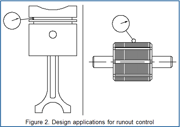
Why Do We Use It? – In precision assemblies, runout causes misalignment and/or balance problems. In Fig. 2, runout of the ring groove diameters relative to the piston’s diameter might cause the ring to squeeze unevenly around the piston or force the piston off center in its bore. A motor shaft that runs out relative to its bearing journals will cause the motor to run out-of-balance, shortening its working life. A designer can prevent such wobble and lopsidedness by specifying a runout tolerance.
The Tolerance call out: A circular runout tolerance is specified using a feature control frame displaying the characteristic symbol. As illustrated in Fig. 3, the arrowhead may be drawn filled or unfilled. The feature control frame includes the runout tolerance value followed by 1 or 2 (but never 3) datum references.

How Does It Work? – As shown in Fig. 2, for as long as piston ring grooves and motor shafts have been made, manufacturers have been finding ways to spin a part about its functional axis while probing its surface with a dial indicator. As the indicator’s tip surfs up and down over the undulating surface, its dial swings gently back and forth, visually displaying the magnitude of runout. Thus, measuring runout can be very simple as long as we agree on 3 things:
- What surface(s) establish the functional axis for spinning—datums?
- Where the indicator is to probe?
- How much swing of the indicator’s dial is acceptable?
The whole concept of “indicator swing” is somewhat dated. Draftsmen used to annotate it on drawings as TIR for “Total Indicator Reading.” The Y14.5 standard briefly called it FIR for “Full Indicator Reading.” Then, in 1973, Y14.5 adopted the international term, FIM for “Full Indicator Movement.”
Full Indicator Movement (FIM) is the difference (in millimeters or inches) between an indicator’s most positive and most negative excursions. Thus, if the lowest reading is -0.01mm and the highest is +0.02mm, the FIM (or TIR or FIR) is 0.03mm. Just because runout tolerance is defined and discussed in terms of FIM doesn’t mean runout tolerance can only be applied to parts that spin in assembly. Neither does it require the part to be rotated, nor use of an antique 20th century, jewel-movement, dial indicator to verify conformance. The “indicator swing” standard is an ideal meant to describe the requirements for the surface. Conformance can be verified using a CMM, optical comparator, laser scanning with computer modeling, process qualification by SPC, or any other method that approximates the ideal.
Considering the purpose for runout tolerance and the way it works, there’s no interaction between a feature’s size and its runout tolerance that makes any sense. In our piston ring groove diameter example from fig.2, an MMC modifier would be counterproductive, allowing the groove diameter’s eccentricity to increase as it gets smaller. That would only aggravate the squeeze and centering problems we’re trying to correct. Thus, material condition modifier symbols, MMC and LMC, are prohibited for both circular and total runout tolerances and their datum references. If you find yourself wishing you could apply a runout tolerance at MMC, you’re not looking at a genuine runout tolerance application; you probably want positional tolerance instead.
Tolerated geometry elements:
Datums for Runout Control = A runout tolerance controls surface elements of a round feature relative to a datum axis. GD&T modernized runout tolerancing by applying the rigors and flexibility of the DRF (Datum Reference Frame). Every runout tolerance shall reference a datum axis. Fig. 4 shows 3 different methods for doing this.

Since a designer wishes to control the runout of a surface as directly as possible, it’s important to select a functional feature(s) to establish the datum axis. During inspection of a part such as that shown in Fig. 4 (a), the datum feature might be placed in a V-block or fixtured in a precision spindle so that the part can be spun about the axis of the datum feature’s TGC (True Geometric Counterpart). This requires that the datum feature be long enough and that its form be well controlled (perhaps by its own size limits or form tolerance). In addition, the datum feature must be easily accessible for such fixturing or probing.
Where a single datum feature or co-datum feature pair establishes the axis, further datum references are meaningless and confusing. However, there are applications where a shoulder or end face exerts more leadership over the part’s orientation in assembly while the diametral datum feature merely establishes the center of revolution. In Fig. 4(c), for example, the face is identified as primary datum feature A and the bore is labeled secondary datum feature B. In inspection, the part will be spun about datum axis B which, remember, is restrained perpendicular to datum plane A. A run-out deviation which can make the testing stylus to move, can have 2 different causes (see Figure 11 below, except for the axial runout b):
• The measured cross-section is not rounded.
• The tolerated form feature is not coaxial.
The circular runout deviation results from the overlaping of circularity and concentricity deviation, therefore is not simply as addition. In this case the dependecies are quite complex.
Circular Runout and Circularity: The perimeter of the tolerated circular cross-section in Figure 11a must lie entirely within the tolerance zone, which – like the circularity tolerance zone – forms a circular ring with a width of tCRo = 0.1 mm. From here the following rule applies:
RULE #1 = Runout tolerance and circularity: In the runout tolerance, the roundness (circularity/circular shape) of all cross-sections is included, meaning that the circularity deviation cannot be greater than the circular run-out tolerance tCRo.
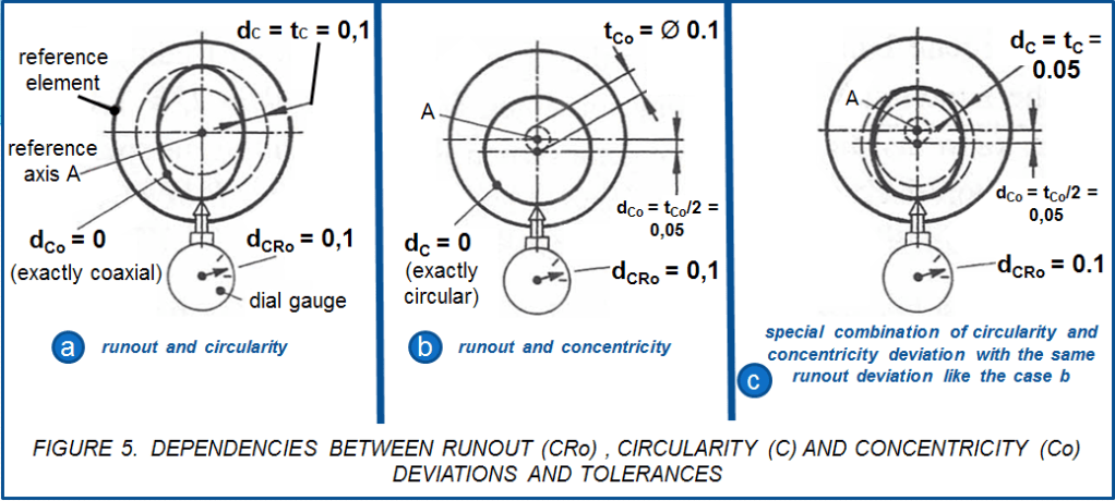
Figure 5 shows a workpiece similar to example (a) from fig.6 (shown below). In limiting case in fig. 5a, the concentricity (coaxiality) deviation between the reference and the tolerated element should be dCO= 0. A circularity tolerance of tC = 0.1 mm is specified for the journal, which use it fully. Such deviations can occur approximately if the workpiece is machined on a worn lathe machine (with circularity deviation) in one setting (without concentricity deviation). The dial gauge obviously deflects by the amount of circular runout tolerance dCRO = tC = 0.1 mm. This gives the next rule:
RULE #2 = Runout and Circularity deviations: When there is no concentricity deviation, the measured runout deviation is equal to the circularity deviation.
Circularity measuring devices respectively form measuring devices work according to this principle. They compensate for coaxiality deviations mathematically or mechanically by aligning the reference axis.
Circular Runout and Concentricity tolerance: = In the other limiting case, Figure 5b, the tolerated cross-section should not have a circularity deviation dC, but a coaxiality deviation (axis offset) dCo; this is equal to the limit deviation tCo/2= 0.05 mm, meaning it makes full use of the specified concentricity tolerance tCo= 0.1 mm. Such deviations can be encountered when the workpiece is re-clamped in a worn lathe machine (with an offset) from a very good lathe (without circularity deviation). The dial gauge again shows a runout deviation of dCRo = 0.1 mm.
RULE # 3 = Runout tolerance and concentricity: If the tolerated cross-section is accurately circular, then the radial runout deviation dCRo is twice as large as the axis offset, just like the concentricity deviation dCo. So if circularity deviations are negligible, the runout tolerance tCRo includes the concentricity with the same tolerance value.In other words: the circular runout tolerance corresponds to a concentricity tolerance with the same tolerance value as long as there are no deviations from the circular shape.
In practice, there will always be a concentricity deviation in addition to the circularity deviation. This usually increases the measured runout deviation,(at least does not decreases it). In Figure 5 the case c is actualy the case b additionally accompanied by a circularity deviation dC = 0.05 mm. Nevertheless, in this case the displayed runout deviation remains, as the greatest difference in the distances to the reference axis A, at dCRo = 0.1 mm (as in case b).
However, it is also possible that the additional circularity deviation to make the measured runout deviation smaller. With an ideally circular cross-section, the concentricity deviation is equal to half the runout deviation (see rule #3). Practical measurements and my own investigations have shown that under real conditions the actual concentricity deviation can be greater than half the measured circular runout deviation by a deviation factor U ~ 1.1 to 1.2; in special cases, U can theoretically even approach the value 2. Figure 6 explains the relationships based on two idealized cross-section profiles.

Nominal constant thickness profiles often resemble the profile in Figure 6a. It has 3 lines of symmetry and consists of 6 circular arcs with 2 different radii r and R, which emanate from the corner points of an internal equilateral triangle (or ideal 3-arc equidistance). Calculations show that the largest excess factor with U = 1.1547 occurs when the reference axis A is in a corner point; in this case, dCo = 0.058 mm (instead of 0.05 mm as in Figure 5(b)). This does not depend on the ratio of the concentricity deviation dCo to the uniform thickness s (where s = r + R), meaning that this exceeding can also occur with small values for axis offset and circularity deviation.
In the case of profiles with 2 lines of symmetry (e.g. ellipses, see Figure 5a), there is no exceeding (i.e. U = 1), but this can happen in the case of profiles with only 1 line of symmetry (mirror symmetry), for example as in Figure 6b . In this case, the excess factor U can theoretically reach a value of 2, while under more practical conditions it is around 1.1 to 1.2. In contrast to the 3-sided profiles, the results here also depend on the calculation of the profile center point M. For this there is still a need for further measurement results and standardization. In summary, we must proceed with the following 2 rules:
RULE #4 = Included tolerances for circular runout: In the circular runout tolerance tCRo the circularity tolerance tC is included with the same tolerance value. The concentricity tolerance tCo, however, is only with an exceeding factor U. Currently, U ~ 1.2 appears to be a usable value (but not U = 1, as is often assumed).
RULE # 5 = Runout instead of coaxiality test: If instead of a specified concentricity tolerance tCo, the circular runout is checked, then the permissible runout deviation is:
dCRo ≤ tCo/U (with U ≈ 1.2)
Note: If a circularity tolerance tC and a concentricity tolerance tCo are specified, the runout deviation dCRo, cannot be greater than their sum: dCRo ≤ tC+tCo
Runout in any direction, circularity and concentricity: With a measuring angle ɑ (acc. to Figure 11 c and d; where d has ɑ = 60°), each individual tolerance zone forms a cone with the angle of inclination ɑ. However, since circularity and concentricity are always checked perpendicular to the reference axis, the included runout tolerances must be slightly modified for any runout direction according to the above rules #1 to #5. If a runout tolerance tCRo is specified, then the following formula applies (according to rules #1 to #5):
Circularity deviation: dC ≤ tCRo/sin ɑ
Concentricity deviation: dCo≤ U*tCRo/2sin ɑ
GD&T Tolerance Zone
The 2-Dimensional circular tolerance zone is an area that is defined by a datum axis where all points on the called surface must fall into. The zone is a direct reference to the datum feature. Circular Runout is the total variation that the reference surface can have when the part is rotated around the datum’s true axis. (as shown in figure 7)

For deviations the following general rule applies:
RULE #6 = Runout deviations: The nominal deviation coresponds to the largest one that occur as display difference during the measurement (apart from the inaccuracy of the measuring device). The limit deviation is equal to the runout tolerance.
When the Circular RunOut tolerance is used?
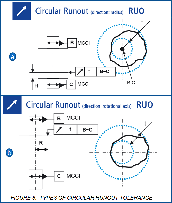
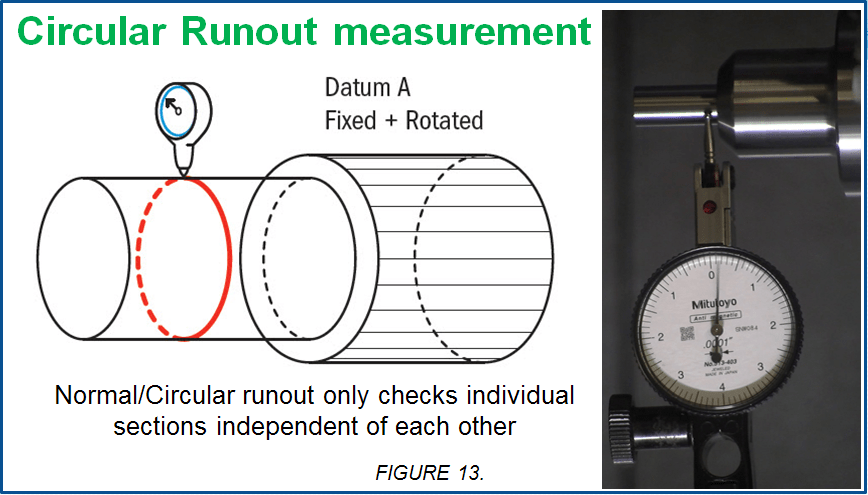
Circular Runout tolerance is the lesser level of runout control. Its tolerance applies to the FIM (Full Indicator Reading) while the indicator probes over a single circle on the part surface. That means the indicator’s body is to remain stationary both axially and radially relative to the datum axis as the part is spun at least 360° about its datum axis. The tolerance applies at every possible circle on the feature’s surface, but each circle may be evaluated separately from the others. Therefore we have 2 types of such cases as shown in Figure 8 below:
- a) Circular Runout on radius
- b) Circular Runout on axis
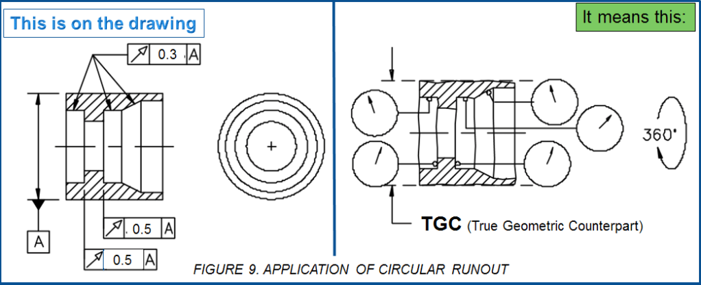
Circular runout can be applied to any feature that is nominally cylindrical, spherical, toroidal, conical, or any revolute having round cross sections (perpendicular to the datum axis). When evaluating noncylindrical features, the indicator shall be continually realigned so that its travel is always normal to the surface at the subject circle. See Fig. 9. Circular runout can also be applied to a face or face groove that is perpendicular to the datum axis. Here, the surface elements are circles of various diameters, each concentric to the datum axis and each evaluated separately from the others.
Runout examples of use:
Example 1: Two coaxial features establishing a datum axis for runout control
Let’s evaluate the 0,5mm circular runout tolerance of Fig.10. We place an indicator near the left end of the controlled diameter and spin the part 360°. We see that the farthest counterclockwise excursion of the indicator dial reaches -0.1mm and the farthest clockwise excursion reaches +0.2mm. The circular runout deviation at that circle is 0.3mm. We move the indicator to the right and probe another circle. Here, the indicator swings between -0.3mm and +0.1mm. The difference, 0.4mm, is calculated without regard for the readings we got from the first circle. The FIM for each circle is compared with the 0.5mm tolerance separately. Obviously, we can’t spend all day trying to measure infinitely many circles, but after probing at both ends of the feature and various places between, we become confident that no circle along the feature would yield an FIM greater than, perhaps, 0.4. Then, we can conclude the feature conforms to the 0.5mm circular runout tolerance.

There are many cases where the part itself is a spindle or rotating shaft that, when assembled, will be restrained in 2 separate places by 2 bearings or 2 bushings. See Fig. 10. If the 2 bearing journals have ample axial separation, it’s unrealistic to try to fixture on just one while ignoring the other. We could better stabilize the part by identifying each journal as a datum feature and referencing both as equal co-datum features. In the feature control frame, the datum reference letters are placed in a single box, separated by a hyphen. The hyphenated co-datum features work as a team. Neither co-datum feature has precedence over the other. We can’t assume the 2 journals will be made perfectly coaxial. To get a decent datum axis from them, we should add a runout tolerance for each journal, referencing the common datum axis they establish, meaning to apply a Total Runout Tolerance which I discuss more in details in a dedicated article.
Example 2: Circular Runuout – Radial, Axial, In any direction and In a specified direction
Figure 11a)– Circular runout – radial: The tolerance arrow is perpendicular to the reference A. The tolerance zone is initially the gap of 0,1mm by which the tip of the probe can move radially with the tolerance tCRo = 0,1mm. This applies to all points of the circular cross-section; meaning that the rotation turns it into a circular ring with the width of the runout tolerance tCRo .The shape of the tolerance zone corresponds to that of circularity, except that its center is now defined by the reference axis. Since each circular ring is checked individually, the convex or conical form of the lateral surface thus the cylindrical shape is not recorded. (This workpiece has a “long” reference axis.)
Figure 11b)– Circular runout – axial: The tolerance arrow is parallel to reference A-B. Individual circular rings are checked concentrically to the axis. The tolerance zones form individual circular cylinder rings of the axial length of the run-out tolerance tCRo. This will only limit the wobble of the frontal surface but not its flatness; it could be for instance either convex or conical. For this reason its perpendicularity deviation can be bigger than its planar run-out tolerance. (The reference axis is in this case the common axis of the 2 bearing seats)

Figure 11c)– Runout in any direction: The runout is checked in the normal direction on the tolerated surface, meaning on local perpendicular direction. For a mechanical measurement this is the simplest way to do it. This means that any surface of revolution can be tolerated (for instance cone, sphere, fillet). Each individual tolerance zone form a cone; this distinguishes from the roundness (circularity) tolerance which is always circular to the ring perpendicular to the axis. (This is a “short” axis which is not suitable as one-time reference. With the locating surface it forms a reference system that allows both checking and function.)
Figure 11d)- Runout in a specified direction: This is used for instance when a copy template must be tolerated in the direction of associated probe. The measuring direction is entered as angular dimension without tolerance (as nominal angle), which applies as theoretical dimension. It would make sense to enter this theoretical dimension in a square. (In this case the common axis is defined by the 2 forehead centereing surfaces.)
Example 3: Rotating Shaft
As shown in Figure 12, a shaft that is rotated at very high speeds is prone to oscillations if the right edge of the shaft is too far offset from the left side. To control how much wobble this part will have runout is used to ensure that the smaller diameter surface is relatively controlled to datum surface A.
To control this without GD&T would be nearly impossible. The small amount of variation in the shaft, straightness of the shaft, and roundness of the individual surfaces would be unrealistic to control.
With runout, you have your final rotational condition that you want controlled without needing to specify unnecessary tight control on the entire part. By constraining with runout as shown on the drawing you are ensuring that when the shaft rotating, with datum A fixed in housing, the reference surface will not go outside of a perfect central rotation by more than 30 microns. This will ensure that only a limited vibration is made and that both parts will wear evenly. To ensure this condition is met, you must measure the parts with a gauge.
B is now controlled in relation to A, ensuring a smooth, near-perfect rotational system.
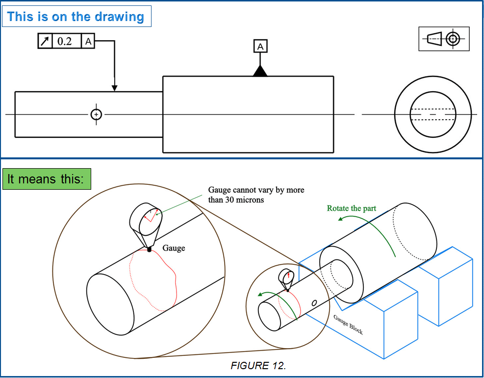
Note: this runout must be controlled on any cross-section along the reference surface. You must gauge each cross-section separately though (Gauging the entire cylinder at once would be Total Runout).
Gauging / Measurement
Runout is measured using a simple height gauge on the reference surface. The datum axis is controlled by fixing all datum points and rotating the central datum axis. The part is usually constrained with V-blocks, or a spindle, on each datum that is required to be controlled. The part is then rotated around this axis and the variation is measured using the height gauge held perpendicular to the part surface. As long as the gauge does not vary by more than the runout tolerance, the part is in spec.
Geometry elements and checking: Runout tolerances are only applicable to rotationally symmetrical parts.
All runout tolerances have an axis (axis of rotation) as a reference. During the measurement, the workpiece rotates around this axis while a measuring device (dial gauge, precision gauge) is placed on the surface to be tested. Nominal features with a circular cross-section (cylinders, cones, etc.) and plane surfaces (frontal surfaces of revolution) are therefore always tolerated. Of course, the measuring device can also rotate around the workpiece. The reference axes have the runout tolerances in common with the coaxiality tolerance. The tolerated area, e.g. the cone or the frontal surface of a shaft must comply with the running tolerance at all points:
RULE # 7 = Testing of the circular runout: The runout is to be checked at a sufficient number of individual positions. Each individual measurement result is compared with the limit deviation (i.e. with the runout tolerance tCRo).
As it is said in practice, between the measurements “the clock is again reset to zero” . Because each individual measurement checks a circular ring of the toleranced element, hence the designation “circular runout” in ISO 1101.
Relation to Other GD&T Symbols
RunOut tolerances have circular tolerance zones of various shapes; therefore they are related to Circularity and Concentricity tolerances.
A great way to relate this symbol to others is through this equation:
Circular Runout = Total Circularity (out of round) + Concentricity (axis offset)

Runout captures both of these in a single measurement when you are comparing the surface to another datum. Runout can also be constrained using a face as well as another circular surface. If this is the case the perpendicularity of the datum face to the reference surface can add into the runout of the surface as well, since if the part is tilted at an angle, the part would runout higher due to the tilting of the part.
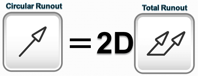
Circular Runout is the 2D version of Total Runout. While it is measured in individual cross-sections, total runout takes the measurement around and across the surface of the entire part in a 3D tolerance zone.
Final Notes
Circular Name: Runout as a GD&T symbol is often referred to as circular runout to differentiate it from total runout.
Two similar versions: Runout is a relation of surface to datum surface or surface to datum axis. When the datum is a surface, any out of round on the datum surface can impact the runout of the part, depending on if the high and low spots on the datum correspond to the high and low spots on the reference feature. (Remember relating the axis to a datum axis is Concentricity)
Regardless of Feature Size: Circular Runout is always RFS (Regardless of Feature Size) meaning that the boundary formed by the dimensions is the entire part envelope that the part can exist regardless of how large the tolerance is. No MMC or bonus tolerance is ever used with it.

Fantastic arguments presented in the article. The author have done a good job at convincing me. Thanks for sharing this.
LikeLike
good to hear this and You’re welcome. It’s my pleasure.
LikeLike